Multiplexing B
from IPython.core.display import HTML
import numpy as np
import matplotlib
import scipy
from scipy.stats import norm
from scipy.stats import binom
from scipy.stats import poisson
import pandas as pd
params = {'figure.figsize':(12,6), # These are plot parameters
         'xtick.labelsize': 16,
         'ytick.labelsize':16,
         'axes.titlesize':18,
         'axes.labelsize':18,
         'lines.markersize':4,
         'legend.fontsize': 20}

from matplotlib import pyplot as plt
matplotlib.rcParams.update(params)
import random
from ipywidgets import *

print('The libraries loaded successfully')
The libraries loaded successfully
This chapter discusses useful approximation results: it provides other illustrations of the CLT, shows how the exponential distribution approaches the geometric distribution, and how the Poisson distribution approaches the binomial distribution.
Central Limit Theorem
Our goal is to illustrate the CLT (see 3.3 in Chapter 3 of this notebook) that we recall here:
Theorem (CLT) Let \(Y_1, Y_2, \ldots\) be independent and identically distributed random variables with mean \(\mu\) and variance \(\sigma^2\). Let also \(X(N) = Y_1 + \cdots + Y_N\). Then
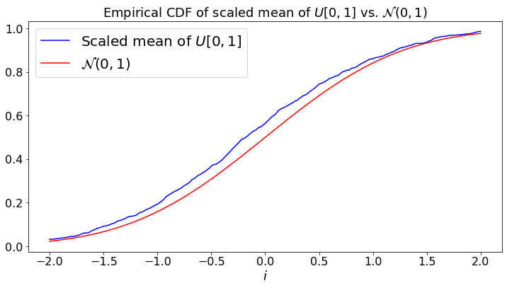
To demonstrate this result, we perform brute-force simulations. We generate \(M \gg 1\) times the random variables \(\{Y_1, \ldots, Y_N\}\) and we compute \(Z = (X(N)/N - N \mu)/(\sigma \sqrt{N})\). We then plot the empirical cumulative distribution \(F(x) = (1/M) \sum_m 1\{Z_m \leq x\} \) where \(Z_m\) is the value of \(Z\) during simulation \(m\). We then compare \(F(x)\) and the cdf of a \({\cal N}(0,1)\) random variable.
We do this in three cases: In case (a), the \(Y_n\) are \(U[0, 1]\); in case (b), they are \(U\{1, 2, \ldots, 6\}\); in case (c), they are \(Expo(1)\).
def dummy(Nd,cased):
    global N, case
    N, case = int(Nd), str(cased)
Nd = widgets.Dropdown(options=['10', '50', '100', '150','200','250','300','350','500'],value='300',description='N',disabled=False)
cased = widgets.ToggleButtons(options=['(a)', '(b)','(c)'],description='Case:',disabled=False,button_style='info',tooltip='Description')

z = widgets.interactive(dummy, Nd = Nd,cased=cased)
display(z)
def CLT3_demo(case,N):
    M = 1000
    S = 100
    a = np.arange(0.0, 2*S + 1)
    b = np.arange(0.0, 2*S + 1)
    c = np.arange(0.0, 2*S + 1)

    if case == '(a)':
        mu = 0.5
        sigma = np.sqrt(1/12)
        L = "$U[0, 1]$"
    elif w == '(b)':
        mu = 3.5
        L = "$U\{1,\ldots,6\}$"
        sigma = 1.7
    else:
        mu = 1
        sigma = 1
        L = "$Expo(1)$"
    z = np.arange(0.0,M+1)
    for m in range(0,M+1):
        y = 0.0
        for n in range(0,N-1):
            if case == '(a)':
                y = y + np.random.random()
            elif w == '(b)':
                y = y + np.random.randint(1,7)
            elif w == '(c)':
                y = y + np.random.exponential(1)
        z[m] = (y - N*mu)/(sigma*N**0.5)
    b[0] = 0.0
    for i in range(0,2*S+1):
        a[i] = 2*i/S - 2
        b[i]=0.0
        for m in range(0,M+1):
            if z[m] <= a[i]:
                b[i] = b[i]+1.0
        b[i] = b[i]/M
        c[i] = norm.cdf(a[i],0,1)
    plt.plot(a, b, color='b',label="Scaled mean of "+ L)
    plt.plot(a, c, color='r',label="${\cal N}(0,1)$")
    plt.legend()
    plt.xlabel("$i$")
    plt.title("Empirical CDF of scaled mean of " +L + " vs. ${\cal N}(0,1)$")

CLT3_demo(case,N)
Characteristic Function
Our main tool in this chapter is the characteristic function.
Definition:
The characteristic function \(\phi_X\) of a random variable \(X\) is defined by
In this expression, \(f_X(x)\) is the pdf of \(X\).
Thus, \(\phi_X\) is the Fourier Transform of \(f_X\).
Here are a few properties of the characteristic function.
Theorem: Properties of the Characteristic Function
(a) \(\phi_X\) characterizes uniquely \(f_X\).
(b) If \(\phi(X_n) \to \phi(X)\) as \(n \to \infty\), then \(X_n \Rightarrow X\).
(c) If \(X\) and \(U\) are independent, then \(\phi_{X + Y}(u) = \phi_X(u)\phi_Y(u)\).
(d) \(\phi^\prime_X(0) = iu E(X)\).
(e) \(\frac{d^k}{dx^k} \phi_X(0) = (iu)^k E(X^k)\).
Note on Proofs:
(c), (d), (e) are obvious. (a) is a property of the Fourier Transform. It says that if two functions have the same Fourier Transform, then they are identical. In (b), \(X_n \Rightarrow X\) means that the cdf of \(X_n\) converges to that of \(X\). The proof of that result is not easy.
Examples:
(a) If \(X =_D {\cal N}(\mu,\sigma^2)\), then \(\phi_X(u) = \exp \{i u \mu - \frac{1}{2} u^2 \sigma^2\}\).
(b) If \(X =_D B(p)\), then \(\phi_X(u) = 1 + p(e^{iu} - 1)\).
(c) If \(X =_D B(n,p)\), then \(\phi_X(u) = [1 + p(e^{iu} - 1)]^n\).
(d) If \(X =_D G(p)\), then \(\phi_X(u) = pe^{iu}[1 - (1 - p)e^{iu}]^{-1}\).
(e) If \(X =_D Expo(\lambda)\), then \(\phi_X(u) = \frac{\lambda}{\lambda - iu}\).
(g) If \(X =_D P(\lambda)\), then \(\phi_X(u) = \exp\{\lambda(e^{iu} - 1)\}\).
Approximation Results
Here are a few useful approximations.
Theorem: As \(n \to \infty\),
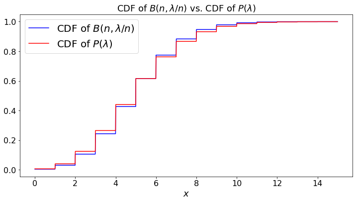
(a) \(B(n, \frac{\lambda}{n}) \Rightarrow P(\lambda)\);
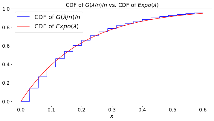
(b) \(\frac{1}{n}G(\frac{\lambda}{n}) \Rightarrow Expo(\lambda)\);
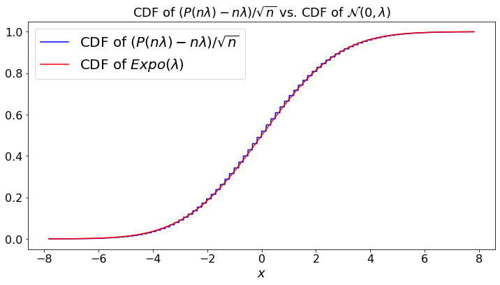
(c) \(\frac{1}{\sqrt{n}}(P(n \lambda) - n \lambda) \Rightarrow {\cal N}(0, \lambda^2)\);
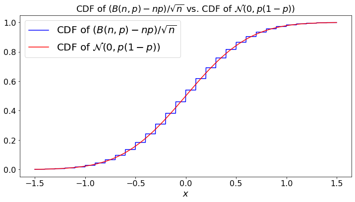
(d) \(\frac{1}{\sqrt{n}}(B(n, p) - np) \Rightarrow {\cal N}(0, p(1-p))\);
Proof:
The book proves these results. To illustrate the method, here is a proof of (a). Using Example (c), the characteristic function of \(B(n, \frac{\lambda}{n})\) is \([1 + (\lambda/n)(e^{iu} - 1)]^n\). Since \((1 + x/n)^n \to \exp\{x\}\), this characteristic function converges to \(\exp\{\lambda(e^{iu} - 1)\}\), which is the characteristic function of \(P(\lambda)\), by Example (e).
Note that (c) follows from the CLT because \(P(n \lambda)\) is distributed like the sum of \(n\) independent \(P(\lambda)\) random variables.Similarly, (d) follows from the CLT and the fact that \(B(n,p)\) is distributed like the sum of \(n\) independent \(B(1,p)\) random variables.
The plots below illustrate these results. For each example, we plot the CDF of the random variables indexed by \(n\) versus the limiting CDF.
def dummy(Nd,Ld):
    global N, L
    N, L = int(Nd), float(Ld)
Nd = widgets.Dropdown(options=['10', '15', '20', '25','30','35','40','50','60'],value='35',description='N',disabled=False)
Ld = widgets.Dropdown(options=['0.1', '0.4', '0.7', '1','2','3','4','5','6','7','8','9','10'],value='5',description='$\lambda$',disabled=False)


z = widgets.interactive(dummy, Nd = Nd,Ld=Ld)
display(z)
def CONV_a(n,L):
    lamb = L
    S = 2000
    a = np.arange(0.0, S)
    c = np.arange(0.0, S)
    d = np.arange(0.0, S)
    for i in range(0,S):
        a[i] = 3*lamb*i/S
        c[i] = poisson.cdf(a[i],lamb)
        d[i] = binom.cdf(a[i], n, lamb/n)
    plt.plot(a, d, color='b',label="CDF of $B(n, \lambda/n)$")
    plt.plot(a, c, color='r',label="CDF of $P(\lambda)$")
    plt.legend()
    plt.xlabel("$x$")
    plt.title("CDF of $B(n,\lambda/n)$ vs. CDF of $P(\lambda)$")

CONV_a(N,L)
def dummy(Nd,Ld):
    global N, L
    N, L = int(Nd), float(Ld)
Nd = widgets.Dropdown(options=['10', '15', '20', '25','30','35','40','50','60'],value='35',description='N',disabled=False)
Ld = widgets.Dropdown(options=['0.1', '0.4', '0.7', '1','2','3','4','5','6','7','8','9','10'],value='5',description='$\lambda$',disabled=False)


z = widgets.interactive(dummy, Nd = Nd,Ld=Ld)
display(z)
def CONV_b(n,L):
    S = 2000
    a = np.arange(0.0, S)
    c = np.arange(0.0, S)
    d = np.arange(0.0, S)
    for i in range(0,S):
        a[i] = (3*i)/(L*S)
        c[i] = scipy.stats.expon.cdf(a[i]*L)
        d[i] = scipy.stats.geom.cdf(int(a[i]*n),float(L/n))
    plt.plot(a, d, color='b',label="CDF of $G(\lambda/n)/n$")
    plt.plot(a, c, color='r',label="CDF of $Expo(\lambda)$")
    plt.legend()
    plt.xlabel("$x$")
    plt.title("CDF of $G(\lambda/n)/n$ vs. CDF of $Expo(\lambda)$")

CONV_b(N,L)
def dummy(Nd,Ld):
    global N, L
    N, L = int(Nd), float(Ld)
Nd = widgets.Dropdown(options=['10', '15', '20', '25','30','35','40','50','60'],value='35',description='N',disabled=False)
Ld = widgets.Dropdown(options=['0.1', '0.4', '0.7', '1','2','3','4','5','6','7','8','9','10'],value='5',description='$\lambda$',disabled=False)


z = widgets.interactive(dummy, Nd = Nd,Ld=Ld)
display(z)
def CONV_c(n,L):
    lamb = L
    S = 2000
    a = np.arange(0.0, S)
    c = np.arange(0.0, S)
    d = np.arange(0.0, S)
    for i in range(0,S):
        a[i] = 3.5*lamb**0.5*(2*i - S)/S
        c[i] = norm.cdf(a[i], 0, lamb**0.5)
        d[i] = poisson.cdf(n**0.5*a[i] + n*lamb, n*lamb)
    plt.plot(a, d, color='b',label="CDF of $(P(n \lambda) - n \lambda)/\sqrt{n}$")
    plt.plot(a, c, color='r',label="CDF of $Expo(\lambda)$")
    plt.legend()
    plt.xlabel("$x$")
    plt.title("CDF of $(P(n \lambda) - n \lambda)/\sqrt{n}$ vs. CDF of ${\cal N}(0,\lambda)$")

CONV_c(N,L)
def dummy(pd, Nd):
    global p, N
    p, N = float(pd), int(Nd)
pd = widgets.Dropdown(options=['0.1', '0.2', '0.3','0.4','0.5','0.6','0.7','0.8','0.9'],value='0.5',description='p',disabled=False)
Nd = widgets.Dropdown(options=['10', '30', '50', '70','100','150','200','250'],value='100',description='N',disabled=False)

z = widgets.interactive(dummy, pd = pd, Nd = Nd)
display(z)
def CONV_d(n,p):
    sig = (p*(1-p))**0.5
    S = 2000
    a = np.arange(0.0, S)
    c = np.arange(0.0, S)
    d = np.arange(0.0, S)
    for i in range(0,S):
        a[i] = 3*sig*(2*i - S)/S
        c[i] = norm.cdf(a[i], 0, sig)
        d[i] = binom.cdf(n**0.5*a[i] + n*p, n, p)
    plt.plot(a, d, color='b',label="CDF of $(B(n,p)-np)/\sqrt{n}$")
    plt.plot(a, c, color='r',label="CDF of ${\cal N}(0, p(1-p))$")
    plt.legend()
    plt.xlabel("$x$")
    plt.title("CDF of $(B(n,p)-np)/\sqrt{n}$ vs. CDF of ${\cal N}(0, p(1-p))$")

CONV_d(N,p)