PageRank B
Comments
This chapter continues our exploration of discrete time Markov chains. In particular, it studies the convergence of the fraction of time that a Markov chain spends in the states and also the convergence of the probability of being in the states. We start with coin flips before moving to Markov chains.
Law of Large Numbers for Coin Flips
You flip a biased coin \(N\) times. The probability of heads is \(p\). Let \(X(N)\) be the number of heads. Then,
Recall that \({N \choose n} = N!/(n!(N - n)!)\) where \(m! = 1\times 2 \times \cdots \times m\) and \(0! := 1\). The expression above is the binominal distribution with parameters \(N\) and \(p\) and we write \(X(N) =_D B(N,p)\).
We plot this distribution:
from IPython.core.display import HTML
import numpy as np
import matplotlib
import scipy
from scipy.stats import norm
from scipy.stats import binom
import pandas as pd
params = {'figure.figsize':(12,6), # These are plot parameters
         'xtick.labelsize': 16,
         'ytick.labelsize':16,
         'axes.titlesize':18,
         'axes.labelsize':18,
         'lines.markersize':4,
         'legend.fontsize': 20}
matplotlib.rcParams.update(params)
from matplotlib import pyplot as plt
import random
from ipywidgets import *

print('The libraries loaded successfully')
The libraries loaded successfully
We display the widgets to select parameters.
def dummy(pd, Nd):
    global p, N
    p, N = float(pd), int(Nd)
pd = widgets.Dropdown(options=['0.1', '0.2', '0.3','0.4','0.5','0.6','0.7','0.8','0.9'],value='0.5',description='p',disabled=False)
Nd = widgets.Dropdown(options=['10', '30', '50', '70','100','150','200','250'],value='100',description='N',disabled=False)

z = widgets.interactive(dummy, pd = pd, Nd = Nd)
display(z)
def IplotBinomial(N,p):
    fig, ax = plt.subplots()
    plt.xlabel("$n$")
    plt.title('Binomial p.m.f. with parameters N = ' + str(N) + ' and p = ' + str(p))
    x = np.arange(N)
    ax.plot(x, binom.pmf(x, N, p), 'bo', ms=4)
    ax.grid(True)
    plt.show()
matplotlib.rcParams.update(params)
IplotBinomial(N,p)
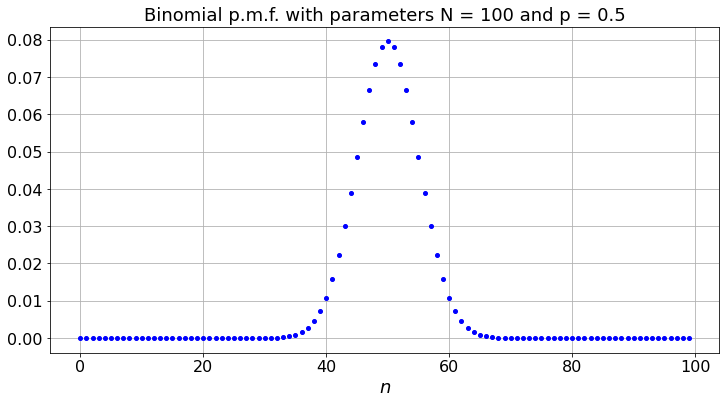
The figure shows that it is unlikely that \(X(N)/N\) differs much from \(p\), specially when \(N\) is large. In fact, a bit of algebra based (2.1) shows that, for any given \(\epsilon > 0\),
where \(A > 0\) and \(\alpha > 0\) are constants that do not depend on \(N\).
The book proves a similar inequality in section 2.2.
We will use this fact to prove the following remarkable property:
Theorem (SLLN)
One has
The figure below illustrates that property, called the Strong Law of Large Numbers.
def dummy(pd, Nd):
    global p, N
    p, N = float(pd), int(Nd)
pd = widgets.Dropdown(options=['0.1', '0.2', '0.3','0.4','0.5','0.6','0.7','0.8','0.9'],value='0.5',description='p',disabled=False)
Nd = widgets.Dropdown(options=['10', '30', '50', '70','100','150','200','250'],value='100',description='N',disabled=False)

z = widgets.interactive(dummy, pd = pd, Nd = Nd)
display(z)
def SLLN_demo(N,p):
    a = np.arange(0.0,N)
    b = np.arange(0.0,N)
    c = np.arange(0.0, N)
    b[0]= np.random.binomial(1,p)
    c[0] = p
    for i in range(0,N-1):
        b[i+1] = (b[i]*(i+1) + np.random.binomial(1,p))/(i+2)
        c[i+1] = p
    colours = ["b","g","r"]
    plt.plot(a, b, color=colours[1],label="simulation")
    plt.plot(a, c, color=colours[2],label="p")
    d = [0, N/10, 2*N/10, 3*N/10, 4*N/10, 5*N/10, 6*N/10, 7*N/10, 8*N/10, 9*N/10, N]
    plt.xticks(d)
    plt.legend()
    plt.ylabel("Fraction")
    plt.xlabel("$n$")
    plt.title("Fraction of heads in $n$ flips, for $n = 1, \ldots, N$")

SLLN_demo(N,p)
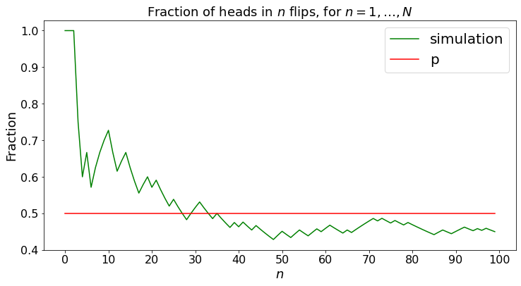
The SLLN says that, as you keep on flipping the coin, the fraction \(X(N)/N\) approaches \(p\), for any experiment. The inequality (2.1) says that for most experiments \(X(N)/N\) is close to \(p\). The SLLN says that for all experiments, \(X(N)/N\) gets closer and closer to \(p\).
The proof of this result is based on the lemma below.
Borel-Cantelli: Don’t Push Your Luck!
This result says that your luck will run out if you push it too far!
Borel-Cantelli Lemma: Assume that event \(n\) occurs with probability \(p_n\), for \(n = 1, 2, \ldots\). If \(\sum_{n=1}^\infty p_n < \infty\), then only finitely many of the events occur. Moreover, if the events are independent and if \(\sum_n p_n = \infty\), then infinitely many of the events occur. See the book for a proof of the lemma.
As an example, say that coin \(n\) has a probability \(p_n\) of heads. We flip the coins \(0, 1, 2, \ldots, n\) and collect \(X_n\) heads. The B-C lemma says that if \(\sum_n p_n < \infty\), then \(X_n\) eventually stops growing and that \(X_n \to \infty\) if \(\sum_n p_n = \infty\),
We do the experiment below in two cases:
In case (a), \(p_n = 1/(n+1)\)
In case (b), \(p_n 2^{- 0.01n}\) for \(n = 0, 1, \ldots\).
def dummy(Nd,cased):
    global N, case
    N, case = int(Nd), str(cased)
Nd = widgets.Dropdown(options=['10', '30', '50', '70','100','150','200','250'],value='100',description='N',disabled=False)
cased = widgets.ToggleButtons(options=['(a)', '(b)'],description='Case:',disabled=False,button_style='info',tooltip='Description')

z = widgets.interactive(dummy, Nd = Nd,cased=cased)
display(z)
def BC_demo(N,case):
    a = np.arange(0.0,N)
    b = np.arange(0,N)
    b[0]= 1
    for n in range(0,N-1):
        if case == '(a)':
            p = 1/(1+n)
        else:
            p = 2**(- 0.01*n)
        b[n+1] = b[n] + np.random.binomial(1,p)
    plt.ylabel("Number X[n] of heads")
    plt.xlabel("$n$")
    plt.title('Number of heads in $n$ flips, for $n = 1, \ldots,$' + str(N) +' for case ' + str(case))
    if case == '(a)':
        label = 'Note that X[n] keeps on increasing'
    else:
        label = 'Note that X(n) eventually stops increasing'
    plt.plot(a, b, color='b',label=label)
    plt.legend()
    d =[0, N/10, 2*N/10, 3*N/10, 4*N/10, 5*N/10, 6*N/10, 7*N/10, 8*N/10, 9*N/10, N]
    d = list(d)
    d = [int(x) for x in d]
    plt.xticks(d)

BC_demo(N,case)
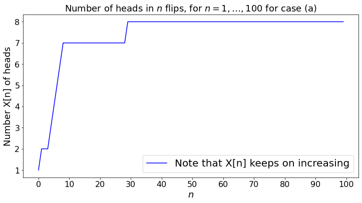
Thus, in case (a), \(\sum_n p_n = \infty\) and, the coin flips being independent, B-C tells us that infinitely many coins yield heads. In case (b), \(\sum_n p_n < \infty\) and B-C states that only finitely many coins yield heads. This result may not be very intuitive: it states that, in case (b), as you keep flipping coins forever, your luck runs out after a finite number of flips and you will never succeed thereafter! (You may have to try (a) a number of times to see that \(X_n\) keeps on growing.)
SLLN and Borel-Cantelli
Let us apply B-C to prove the SLLN for the coin flips.
Using (2.2) and B-C, we see that \(\{|\frac{X(N)}{N} - p| > \epsilon\}\) occurs for finitely many \(N\)’s. Hence, there is some \(N_0\) such that, for all \(N \geq N_0\), one has \(|\frac{X(N)}{N} - p| > \epsilon\). Since \(\epsilon > 0\) is arbitrary, this proves that \(X(N)/N \to p\) as \(N \to \infty\).
SLLN for i.i.d. Random Variables
Let \(Y_1, Y_2, \ldots\) be independent and identically distributed random variables. Let also \(X(N) = Y_1 + \cdots + Y_N\). Then, under a weak condition,
The book proves that result assuming that \(E(Y_1^4) < \infty\). Using that assumption, one shows that
for some constant \(A\) that does not depend on \(N\). Since these probabilities have a finite sum over \(N\), one can use the same argument as for coin flips to prove (2.4).
SLLN for Markov Chains
As we saw in Chapter 1, if a Markov chain is irreducible, the fraction of time it spends in state \(i\) converges to \(\pi(i)\), the invariant probability of that state. Recall that we find \(\pi\) by solving the balance equations \(\pi = \pi P\).
The proof of the theorem looks that the successive times \(\tau, \tau + T_1, \tau + T_1 + T_2, \ldots\) when the Markov chain returns to state \(i\). The random variables \(T_1, T_2, \ldots\) are independent and identically distributed because the Markov chain restarts afresh whenever it enters state \(i\). Consequently, the SLLN holds for these times, and this shows that the time for \(n\) successive visits to state \(i\) is roughly \(n E(T_1)\), which proves that the fraction of time in state \(i\) converges to \(1/E(T_1)\). One can then show that these limiting fractions of time solve the balance equations and, therefore, \(1/E(T_1) = \pi(i)\).