Speech Recognition A
This chapter introduces some basic learning algorithms and then discussed the Viterbi algorithm.
from IPython.core.display import HTML
import numpy as np
import matplotlib
import scipy
from scipy.stats import norm
from scipy.stats import binom
import pandas as pd
params = {'figure.figsize':(12,6), # These are plot parameters
         'xtick.labelsize': 16,
         'ytick.labelsize':16,
         'axes.titlesize':18,
         'axes.labelsize':18,
         'lines.markersize':4,
         'legend.fontsize': 20}
matplotlib.rcParams.update(params)
from matplotlib import pyplot as plt
import random
import math
from ipywidgets import *
import numpy.linalg
from IPython.display import display
from IPython.core.display import HTML
from notebook.nbextensions import enable_nbextension
%matplotlib inline

print('The libraries loaded successfully')
The libraries loaded successfully
Baysian Updates
Bayes’ Rule enables to update beliefs as one makes observations.
Review of Bayes’ Rule
Recall the basic setup. The events \(A_1, \ldots, A_N\) are a partition of the sample space \(\Omega\) and \(B\) is another event. Then one has the following result.
Bayes’ Rule:
This rule extends to continuous random variables. Say that \(X\) takes values in \(\{1, \ldots, N\}\) and that \(P(X = n) = p_n\). Assume also that the random variable \(Y\) has pdf \(f_n(y)\) when \(X = n\). That is, formally, \(f_{Y|X}[y|n] = f_n(y)\). Then
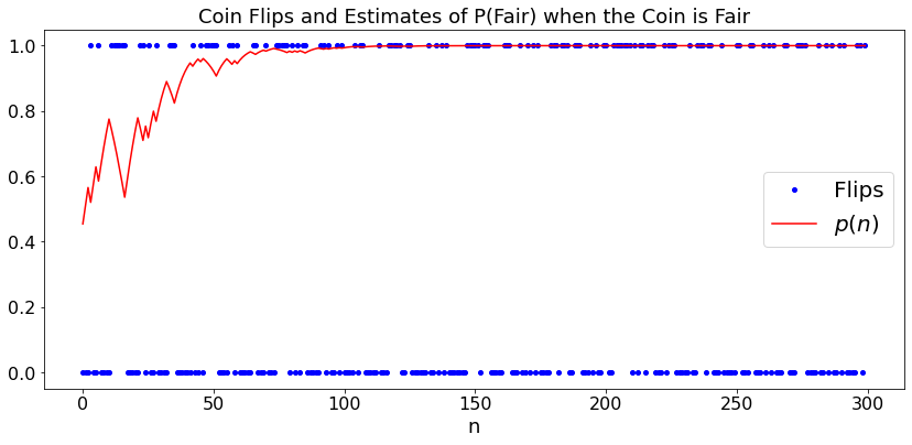
Bias of Coin
As a first example, say that you have a coin that is fair with probability \(p\) and biased with \(P(H) = 0.6\) otherwise. How do you update your estimate of \(p\) as you flip the coin?
Say that you flip the coin once and get \(H\). Then, the probability that the coin is fair is
Similalry,
The formulas above enable us to update our estimate of \(p\) after every coin flip.
Let’s try this. In the plot, \(1\) represents \(H\) and \(0\) represents \(T\).
def dummy(Nd,cased):
    global N, case
    N, case = int(Nd), str(cased)

Nd = widgets.Dropdown(options=['10', '30', '50', '70','100','150','200','250','300','350','400','450','500'],value='300',description='N',disabled=False)
cased = widgets.ToggleButtons(options=['Fair', 'Biased'],description='Case:',disabled=False,button_style='info',tooltip='Description')

z = widgets.interactive(dummy, Nd = Nd, cased=cased)
display(z)
def BU(w,N):  # Simulation of DTMC with initial state w given by button
    a = np.arange(0,N)
    x = np.arange(0,N)
    p = np.arange(0.0,N)
    x[0] = 0
    p[0]=0.5*0.5/(0.5*0.5 + 0.6*0.5)
    if w == 'Fair':
        case_str = 'Fair'
        q = 0.5
    else:
        case_str = 'Biased'
        q = 0.6
    for n in range(1,N):
        x[n] = np.random.binomial(1,q)
        if x[n] == 1:
            p[n] = 0.5*p[n-1]/(0.5*p[n-1] + 0.6*(1 - p[n-1]))
        else:
            p[n] = 0.5*p[n-1]/(0.5*p[n-1] + 0.4*(1 - p[n-1]))

    plt.figure(figsize = (14,6))
    plX, = plt.plot(a,x,'bo',label='Flips')
    plt.legend()
    plp, = plt.plot(a,p,'red',label='$p(n)$')
    plt.legend()
    plt.title('Coin Flips and Estimates of P(Fair) when the Coin is ' + case_str)
    plt.xlabel('n')

BU(case,N)
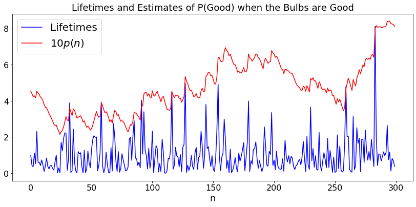
Are these lightbulbs defective?
Assume you have a batch of lightbulbs that are all “good” and have an exponential lifetime with mean \(1\) with probability \(p\). Otherwise, they all have a lifetime that is exponentially distibuted with mean \(0.9\) and are considered “defective”. You observe the lifetimes of successive bulbs and update the probability that they are good.
Let \(x\) be the lifetime of the next bulb. By Bayes’ Rule:
Let us try this. Note that we plot \(10p(n)\) for legibility of the graph.
def dummy(Nd,cased):
    global N, case
    N, case = int(Nd), str(cased)

Nd = widgets.Dropdown(options=['10', '30', '50', '70','100','150','200','250','300','350','400','450','500'],value='300',description='N',disabled=False)
cased = widgets.ToggleButtons(options=['Good', 'Defective'],description='Case:',disabled=False,button_style='info',tooltip='Description')

z = widgets.interactive(dummy, Nd = Nd, cased=cased)
display(z)
def BU(w,N):  # Simulation of DTMC with initial state w given by button
    a = np.arange(0,N)
    x = np.arange(0.0,N)
    p = np.arange(0.0,N)
    x[0] = 1
    p[0]=0.5*0.5/(0.5*0.5 + 0.6*0.5)
    if w == 'Good':
        case_str = 'good'
        q = 1
    else:
        case_str = 'defective'
        q = 0.9
    for n in range(1,N):
        x[n] = np.random.exponential(q)
        A = p[n-1]*math.exp(-x[n])
        p[n] = A/(A + (1 - p[n-1])*math.exp(-x[n]/0.9)/0.9)

    plt.figure(figsize = (14,6))
    plX, = plt.plot(a,x,'blue',label='Lifetimes')
    plt.legend()
    plp, = plt.plot(a,10*p,'red',label='$10p(n)$')
    plt.legend()
    plt.title('Lifetimes and Estimates of P(Good) when the Bulbs are ' + w)
    plt.xlabel('n')

BU(case,N)
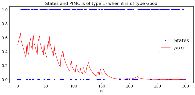
Which Markov Chain is This?
We observe the successive states of a Markov chain. With probability \(p\), the probability transition matrix is \(P_1\) and the initial distribution is \(\pi_1\). Otherwise, they are \(P_2\) and \(\pi_2\), respectively. How do we update \(p\) as we observe more transitions?
Again, we use Bayes’ Rule. Say that we observe \(x_0\). We have
Now assume we have observed \((x_0, \ldots, x_n)\) and have computed the probability \(p_n = P[1|x_0, \ldots, x_n]\). We then observe \(x_{n+1}\). Bayes’ Rule implies that
Let us try this when the state space is \(\{0, 1\}\) and \(\pi_1 = \pi_2 = [0.5, 0.5]\) and \(P_1(0, 1) = P_1(1, 0) = 0.2\) whereas \(P_2(0,1) = 0.3\) and \(P_2(1,0) = 0.1\).
def dummy(Nd,cased):
    global N, case
    N, case = int(Nd), str(cased)

Nd = widgets.Dropdown(options=['10', '30', '50', '70','100','150','200','250','300','350','400','450','500'],value='300',description='N',disabled=False)
cased = widgets.ToggleButtons(options=['Good', 'Defective'],description='Case:',disabled=False,button_style='info',tooltip='Description')

z = widgets.interactive(dummy, Nd = Nd, cased=cased)
display(z)
def BUMC(case,N):  # Simulation of DTMC with initial state w given by button
    a = np.arange(0,N)
    x = np.arange(0,N)
    p = np.arange(0.0,N)
    x[0] = 0
    p[0]=0.5
    if case == '1':
        c = 0
    else:
        c = 1
    P = np.zeros((2,2,2))
    P[0,:,:] = [[0.8,0.2],[0.2,0.8]]
    P[1,:,:] = [[0.7,0.3],[0.1,0.9]]
    for n in range(1,N):
        if x[n-1] == 0:
            x[n] = np.random.binomial(1,P[c,0,1])
        else:
            x[n] = 1 - np.random.binomial(1,P[c,1,0])
        p[n] = p[n-1]*P[0,x[n-1],x[n]]/(p[n-1]*P[0,x[n-1],x[n]] + (1 - p[n-1])*P[1,x[n-1],x[n]])

    plt.figure(figsize = (14,6))
    plX, = plt.plot(a,x,'bo',label='States')
    plt.legend()
    plp, = plt.plot(a,p,'red',label='$p(n)$')
    plt.legend()
    plt.title('States and P(MC is of type 1) when it is of type ' + case)
    plt.xlabel('n')

BUMC(case,N)
Viterbi Algorithm
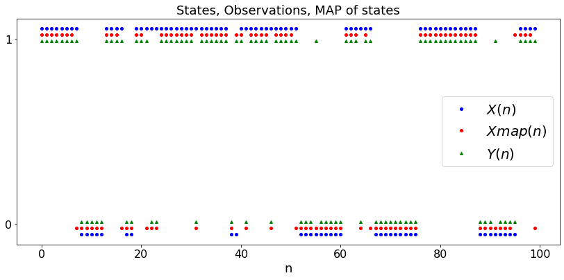
The Viterbi Algorithm calculates the most likely sequence \((x_0, x_1, \ldots, x_n)\) of states of a Markov chain give a sequence \((y_0, y_1, \ldots, y_n)\) of noisy measurements. Here, the Markov chain \(X_n\) has a known initial distribution \(\pi\) and probability transition matrix \(P\). The observations are defined by \(P[Y_n = y | X_0, \ldots X_n] = q(X_n,y)\) where \(q\) is a known matrix.
From Bayes’ Rule, we see that
where \(A\) is a normalization constant that does not depend on \((x_0, \ldots, x_n)\).
Hence, the most likely sequence \((x_0, \ldots, x_n)\) given \((Y_0, \ldots, Y_n)\) is the sequence that maximizes the product \(\pi(x_0)q(x_0, Y_0) P(x_0, x_1) q(x_1, Y_1) \cdots P(x_{n-1}, x_n)q(x_n, Y_n)\). The logarithm of that product is equal to
where \(d_0(\theta, x_0) = - \log (\pi(x_0)q(x_0, Y_0))\) and \(d_m(x_{m-1}, x_m) = - \log(P(x_{m-1}, x_m)q(x_m, Y_m))\). Maximizing this expression is then equivalent to minimizing the sum \(d_0(\theta, x_0) + \sum_{m=1}^n d_m(x_{m-1}, x_m)\) which can be viewed as the length of the path \((\theta, x_0, \ldots, x_n)\). That is, finding the most likely sequence of states is equivalent to finding a shortest path.
We use the Bellman-Ford algorithm to find this shortest path. Let \(V_m(x_m)\) be the length of the shortest path \((x_m, x_{m+1}, \ldots, x_n)\), i.e., the smallest value of \(d_{m+1}(x_m, x_{m+1}) + \cdots + d_n(x_{n-1},x_n)\). By writing the length of the path \((x_{m-1}, x_m, \ldots, x_n)\) as \(d_m(x_{m-1}, x_m)\) plus the length of the path \((x_m, \ldots, x_n)\), and minimizing first over the the path from \(x_m\) and then over \(x_m\), we find that
where \(x_{-1} := \theta\) and \(V_n(x_n) := 0\). We then solve recursively backwards, starting with \(m = n\) and then continuing with \(m = n-1, n-2, \ldots, 0\).
We illustrate the algorithm on the simplest possible example where \(x_n \in \{0, 1\}\) and \(y_n \in \{0, 1\}\). We assume \(P(0, 1) = a, P(1, 0) = b\), \(\pi(0) = b/(a + b)\). Also, \(q(x,y) = 1 - \epsilon\) if \(x = y\) and \(q(x, y) = \epsilon\) if \(x \neq y\).
def dummy(epsd,ad,bd,Nd):
    global eps, a, b, N
    eps, a, b, N = float(epsd), float(ad), float(bd), int(Nd)

epsd = widgets.Dropdown(options=['0.02', '0.04', '0.06', '0.08','0.1','0.12','0.14','0.16','0.18','0.2','0.22','0.24','0.26','0.28','0.3','0.32','0.34','0.36','0.38','0.4','0.42','0.44','0.46','0.48','0.5'],value='0.1',description='$\epsilon$',disabled=False)
ad = widgets.Dropdown(options=['0.02', '0.04', '0.06', '0.08','0.1','0.12','0.14','0.16','0.18','0.2','0.22','0.24','0.26','0.28','0.3','0.32','0.34','0.36','0.38','0.4','0.42','0.44','0.46','0.48','0.5'],value='0.1',description='$a$',disabled=False)
bd = widgets.Dropdown(options=['0.02', '0.04', '0.06', '0.08','0.1','0.12','0.14','0.16','0.18','0.2','0.22','0.24','0.26','0.28','0.3','0.32','0.34','0.36','0.38','0.4','0.42','0.44','0.46','0.48','0.5'],value='0.1',description='$b',disabled=False)
Nd = widgets.Dropdown(options=['10', '30', '50', '70','100','150','200','250'],value='100',description='N',disabled=False)

z = widgets.interactive(dummy, epsd=epsd,ad=ad,bd=bd,Nd=Nd)
display(z)
def VIT(eps,a,b,N):  # Viterbi
    t = np.arange(0,N)
    x = np.arange(0,N)
    xmap = np.arange(0,N)
    y = np.arange(0,N)
    V = np.zeros((N,2))
    d = np.zeros((N,2,2))
    x[0] = np.random.binomial(1,b/(a+b))
    P = np.array([[1-a, a],[b, 1 -b]])
    sd = np.array([b/(a+b), a/(a+b)])
    Q = np.array([[1-eps, eps],[eps, 1-eps]])

    ## simulate MC and observations
    if x[0] == 0:
        y[0] = np.random.binomial(1,eps)
    else:
        y[0]= 1 - np.random.binomial(1,eps)
    for n in range(1,N):
        if x[n-1] == 0:
            x[n] = np.random.binomial(1,a)
        else:
            x[n] = 1 - np.random.binomial(1,b)
        if x[n] == 0:
            y[n] = np.random.binomial(1,eps)
        else:
            y[n]= 1 - np.random.binomial(1,eps)


    ##Belman-Ford Algorithm
    if y[0]== 0:
        c = np.array([1-eps, eps])
    else:
        c = np.array([eps,1 - eps])
    for n in range(1,N):
        for i in range(2):
            for j in range(2):
                d[n,i,j] = - math.log(P[i,j]) - math.log(Q[j,y[n]])
    for n in range(2,N):
        for i in range(2):
            V[N-n,i] = min(d[N-n,i,0]+ V[N-n+1,0],d[N-n,i,1]+ V[N-n+1,1])
    for i in range(2):
        V[0,i] = - math.log(c[i]) - math.log(sd[i]) + V[1,i]
    for n in range(0,N):
        xmap[n]= (V[n,1] < V[n,0])


    plt.figure(figsize = (14,6))
    plx, = plt.plot(t,x,'bo',label='$X(n)$')
    plt.legend()
    plxmap, = plt.plot(t,0.03 + 0.94*xmap,'ro',label='$Xmap(n)$')
    plt.legend()
    plY, = plt.plot(t,0.06+ 0.88*y,'g^',label='$Y(n)$')
    plt.legend()
    labels = ['0', '1']
    plt.yticks([0.05, 0.95], labels)
    plt.title('States, Observations, MAP of states')
    plt.xlabel('n')

VIT(eps,a,b,N)
Clustering
Clustering is a basic process in learning.
Example 1: Student Scores, Same Variance
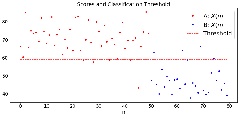
As a simple example, say that you look at the scores of students on a set of exams. You want to classify the students into A = very good and B = not so good. A simple rule would be “not-curved” where you decide that a student is A if her average score is larger than \(80\) and is B otherwise. The “curved” rule is more tricky because you have to choose the threshold based on the observed scores. You may decide that \(30\%\) of the students are \(A\), in which case you adjust the threshold so that this happens. A more subtle approach is to assume that the scores of \(A\) students are \({\cal N}(a, \sigma^2)\) and those of \(B\) students are \({\cal N}(b, \sigma^2)\), but we only know that \(a > b\). In this case, here is an algorithm. Let \(X(1), \ldots, X(n)\) be the scores of the \(N\) students.
Initialize: Let \(z = (X(0) + \cdots + X(n))/(n+1)\);
For \(k = 0, 1, ...\): Define group \(A\) to be students with score larger than \(z(0)\), and group \(B\) to be the other students. Recompute the mean \(a\) of group \(A\) and the mean \(b\) of group \(B\). Define \(z(k+1) = (a + b)/2\).
We try this algorithm by first choosing \((a, b, \sigma)\) and we generate \(M\) random scores that are \({\cal N}(a, \sigma^2)\) and \(N\) that are \({\cal N}(b, \sigma^2)\). We run the algorithm and look at the misclassified students.
def dummy(sigd,ad,bd,Nd,Md):
    global sig, a, b, N, M
    sig, a, b, N, M = float(sigd), float(ad), float(bd), int(Nd), int(Md)

sigd = widgets.Dropdown(options=['1', '2', '3', '4','5','6','7','8','9','10','11','12','13','14','15'],value='8',description='$\sigma$',disabled=False)
ad = widgets.Dropdown(options=['10', '20', '30', '40','50','60','70','80','90','100','110','120','130','140'],value='70',description='$a$',disabled=False)
bd = widgets.Dropdown(options=['10', '20', '30', '40','50','60','70','80','90','100','110','120','130','140'],value='50',description='$b',disabled=False)
Nd = widgets.Dropdown(options=['10', '30', '50', '70','100','150','200','250'],value='30',description='N',disabled=False)
Md = widgets.Dropdown(options=['10', '30', '50', '70','100','150','200','250'],value='50',description='M',disabled=False)


z = widgets.interactive(dummy, sigd=sigd,ad=ad,bd=bd,Nd=Nd,Md=Md)
display(z)
def CLU(sig,a,b,M, N):  # Clustering
    t = np.arange(0,M + N)
    x = np.arange(0.0,M + N)
    y = np.arange(0,M + N)
    ta = np.arange(0,M)
    xa = np.arange(0.0,M)
    tb = np.arange(0,N)
    xb = np.arange(0.0,N)
    S = 40

    ## Generate scores
    for n in range(M):
        x[n] = np.random.normal(a,sig)
        xa[n] = x[n]
    for n in range(N):
        x[n+M] = np.random.normal(b,sig)
        tb[n] = M + n
        xb[n] = x[n+M]
    z = sum(x)/(M+N)
    for s in range(S):
        A = 0
        NA = 0
        B = 0
        NB = 0
        for n in range(N+M):
            if x[n] < z:
                NB = NB + 1
                B = B + x[n]
            else:
                NA = NA + 1
                A = A + x[n]
        z = (B/NB + A/NA)/2
    for n in range(M+N):
        y[n] = z
    print('Guessed a = ', round(A/NA,1),'; Guessed b = ', round(B/NB,1))

    plt.figure(figsize = (14,6))
    plx, = plt.plot(ta,xa,'ro',label='A: $X(n)$')
    plt.legend()
    plx, = plt.plot(tb,xb,'bo',label='B: $X(n)$')
    plt.legend()
    plxmap, = plt.plot(t,y,'r--',label='Threshold')
    plt.legend()
    plt.title('Scores and Classification Threshold')
    plt.xlabel('n')

CLU(sig,a,b,M, N)
Guessed a = 71.9 ; Guessed b = 47.7
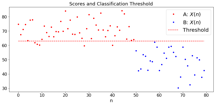
Example 2: Student Scores, Different Variances
The setup is the same, but we now assume that the cores of A-students are \({\cal N}(a, \sigma_a^2)\) and those of B-students are \({\cal N}(b, \sigma_b^2)\). Here is our algorithm:
Initialize: Let \(z = (X(0) + \cdots + X(n))/(n+1)\). Define group A to be students with a score larger than \(z\). Let then \(a\) be the mean of the scores of those students and \(\sigma_a^2\) the sample variance of those scores, similarly for \(b\) and \(\sigma_b^2\).
Steps \(k = 0, 1, \ldots\): \(m\) is of group \(A\) if \(|X_m - a|/\sigma_a < |X_m - b|/\sigma_b\) and is of group \(B\) otherwise. Let \(a\) = mean of group \(A\), \(\sigma_a^2\) = sample variance of group \(B\), similarly for \(b\) and \(\sigma_b^2\).
Here is a simulation. We choose the actual parameters \((a, b, \sigma_a, \sigma_b)\) and the number \(M\) of students of group \(A\) and \(N\) of group \(B\). We run the algorithm and visualize the classification.
def dummy(sigad,sigbd,ad,bd,Nd,Md):
    global siga, sigb, a, b, N, M
    siga, sigb, a, b, N, M = float(sigad), float(sigbd), float(ad), float(bd), int(Nd), int(Md)

sigad = widgets.Dropdown(options=['1', '2', '3', '4','5','6','7','8','9','10','11','12','13','14','15'],value='8',description='$\sigma_a$',disabled=False)
sigbd = widgets.Dropdown(options=['1', '2', '3', '4','5','6','7','8','9','10','11','12','13','14','15'],value='8',description='$\sigma_b$',disabled=False)
ad = widgets.Dropdown(options=['10', '20', '30', '40','50','60','70','80','90','100','110','120','130','140'],value='70',description='$a$',disabled=False)
bd = widgets.Dropdown(options=['10', '20', '30', '40','50','60','70','80','90','100','110','120','130','140'],value='50',description='$b',disabled=False)
Nd = widgets.Dropdown(options=['10', '30', '50', '70','100','150','200','250'],value='30',description='N',disabled=False)
Md = widgets.Dropdown(options=['10', '30', '50', '70','100','150','200','250'],value='50',description='M',disabled=False)


z = widgets.interactive(dummy, sigad=sigad,sigbd=sigbd,ad=ad,bd=bd,Nd=Nd,Md=Md)
display(z)
def CLU2(siga,sigb,a,b,M, N):  # Clustering
    t = np.arange(0,M + N)
    x = np.arange(0.0,M + N)
    y = np.arange(0,M + N)
    ta = np.arange(0,M)
    xa = np.arange(0.0,M)
    tb = np.arange(0,N)
    xb = np.arange(0.0,N)
    S = 40

    ## Generate scores
    for n in range(M):
        x[n] = np.random.normal(a,siga)
        xa[n] = x[n]
    for n in range(N):
        x[n+M] = np.random.normal(b,sigb)
        tb[n] = M + n
        xb[n] = x[n+M]

    z = sum(x)/(N+M)
    A = 0
    NA = 0
    SA = 0
    B = 0
    NB = 0
    SB = 0
    for n in range(N+M):  ## initialize
        if x[n] < z:
            NB = NB + 1
            B = B + x[n]
            SB = SB + x[n]**2
        else:
            NA = NA + 1
            A = A + x[n]
            SA = SA + x[n]**2
    ma = A/NA
    mb = B/NB
    sa = (SA/NA - ma**2)**0.5
    sb = (SB/NB - mb**2)**0.5
    z = (sb*ma + sa*mb)/(sa + sb)

    for s in range(S):  ## Classification
        A = 0
        NA = 0
        SA = 0
        B = 0
        NB = 0
        SB = 0
        for n in range(N+M):
            if x[n] < z:
                NB = NB + 1
                B = B + x[n]
                SB = SB + x[n]**2
            else:
                NA = NA + 1
                A = A + x[n]
                SA = SA + x[n]**2
        ma = A/NA
        mb = B/NB
        sa = (SA/NA - ma**2)**0.5
        sb = (SB/NB - mb**2)**0.5
        z = (sb*ma + sa*mb)/(sa + sb)
    for n in range(M+N):
        y[n] = z
    ma = math.ceil(ma*10)/10
    sa = math.ceil(sa*10)/10
    mb = math.ceil(mb*10)/10
    sb = math.ceil(sb*10)/10
    print('Guessed a = ', ma,'; Guessed sa = ', sa, '; Guessed b = ', mb,'; Gessed sb ', sb)

    plt.figure(figsize = (14,6))
    plx, = plt.plot(ta,xa,'ro',label='A: $X(n)$')
    plt.legend()
    plx, = plt.plot(tb,xb,'bo',label='B: $X(n)$')
    plt.legend()
    plxmap, = plt.plot(t,y,'r--',label='Threshold')
    plt.legend()
    plt.title('Scores and Classification Threshold')
    plt.xlabel('n')

CLU2(siga,sigb,a,b,M, N)
Guessed a = 71.9 ; Guessed sa = 5.8 ; Guessed b = 50.4 ; Gessed sb 8.6
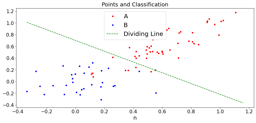
Example 3: 2D Classification
In this example, we generate \(M\) pairs \((X, Y)\) that are distributed like \((a_1, a_2)' + A(v_1, v_2)'\) where \(A\) is a \(2\)-by-\(2\) matrix and \(v_1, v_2\) are independent \({\cal N}(0, 1)\). We also generate \(N\) pairs that are distributed like \((b_1, b_2)' + B(v_1, v_2)'\). We then classify the \(M + N\) points. Here is the classification algorithm:
Initialize: Let \(\{c + dx, x \in \Re\}\) be the linear regression of \(Y\) over \(R\).
Subsequent steps: The points \(A\) are above the line \(\{c + dx, x \in \Re\}\) and the points \(B\) are the other points. Let \(a\) and \(b\) be the mean values of group \(A\) and \(B\), respectively. Let then \(\{c + dx, x \in \Re\}\) be the bisectrice of the segment \((a, b)\).
Here is a simulation. To simplify the user input, we choose \((b_1, b_2) = (0, 0)\) and \((a_1, a_2) = (a, a)\). Also, we specify that \(B\) is the indentity matrix multipled by \(\sigma_b\). Finally, \(A = \sigma_a \times [[1, 0.5], [0.5, 1]]\).
def dummy(sigad,sigbd,ad,Nd,Md):
    global siga, sigb, a,N, M
    siga, sigb, a, N, M = float(sigad),float(sigbd), float(ad), int(Nd), int(Md)

sigad = widgets.Dropdown(options=['0.05', '0.1', '0.15', '0.2','0.25','0.3','0.35','0.4','0.45'],value='0.2',description='$\sigma_a$',disabled=False)
sigbd = widgets.Dropdown(options=['0.05', '0.1', '0.15', '0.2','0.25','0.3','0.35','0.4','0.45'],value='0.2',description='$\sigma_b$',disabled=False)
ad = widgets.Dropdown(options=['0.05', '0.1', '0.15', '0.2','0.25','0.3','0.35','0.4','0.45'],value='0.4',description='$a$',disabled=False)
Nd = widgets.Dropdown(options=['10', '30', '50', '70','100','150','200','250'],value='30',description='N',disabled=False)
Md = widgets.Dropdown(options=['10', '30', '50', '70','100','150','200','250'],value='50',description='M',disabled=False)


z = widgets.interactive(dummy, sigad=sigad,sigbd=sigbd,ad=ad,Nd=Nd,Md=Md)
display(z)
def CLU3(siga,sigb,a,M, N):  # Clustering
    t = np.arange(0,M + N)
    x = np.zeros((2,M + N))
    S = 40
    D = np.array([[1, 0.5],[0.5,1]])

    ## Generate points
    for n in range(N):
        x[:,n] = np.random.normal(0,sigb,2)
    for n in range(M):
        x[:,n+N] = np.dot(D,np.random.normal(a,siga,2))
    sx2 = 0
    sxy = 0
    m = sum(x)/(N+M)
    for n in range(N+M):  ## initialize
        sx2 = sx2 + x[0,n]**2
        sxy = sxy + x[0,n]*x[1,n]
    sx2 = sx2/(N+M) - m[0]**2
    sxy = sxy/(N+M) - m[0]*m[1]
    d = sxy/sx2
    c = m[1] - d*m[0]

    for s in range(S):  ## Classification
        A = np.array([0,0])
        NA = 0
        B = np.array([0,0])
        NB = 0
        for n in range(N+M):
            if x[1,n] < c + d*x[0,n]:
                NB = NB + 1
                B = B + x[:,n]
            else:
                NA = NA + 1
                A = A + x[:,n]
        ma = A/NA
        mb = B/NB
        d = (mb[0] - ma[0])/(ma[1] - mb[1])
        c = (ma[1] + mb[1] - d*(ma[0] + mb[0]))/2

    y = np.zeros((2,100))
    minx = min(x[0,:])
    maxx = max(x[1,:])
    delta = (maxx - minx)/100
    for n in range(100):
        y[0,n] = minx + delta*n
        y[1,n] = c + d*y[0,n]

    plt.figure(figsize = (14,6))
    plxb, = plt.plot(x[0,N:M+N], x[1,N:M+N],'ro',label='A')
    plt.legend()
    plxa, = plt.plot(x[0,0:N], x[1,0:N],'bo',label='B')
    plt.legend()
    ply, = plt.plot(y[0,:],y[1,:],'g--',label='Dividing Line')
    plt.legend()
    plt.title('Points and Classification')
    plt.xlabel('n')


CLU3(siga,sigb,a,M, N)