Route Planning A
from IPython.core.display import HTML
import numpy as np
import matplotlib
import scipy
from scipy.stats import norm
from scipy.stats import binom
import pandas as pd
params = {'figure.figsize':(12,6), # These are plot parameters
         'xtick.labelsize': 16,
         'ytick.labelsize':16,
         'axes.titlesize':18,
         'axes.labelsize':18,
         'lines.markersize':4,
         'legend.fontsize': 20}
matplotlib.rcParams.update(params)
from matplotlib import pyplot as plt
import random
from ipywidgets import *
import numpy.linalg
from IPython.display import display
from IPython.core.display import HTML
from notebook.nbextensions import enable_nbextension
%matplotlib inline

print('The libraries loaded successfully')
The libraries loaded successfully
Stochastic dynamic programming is a methodology for making sequential decisions in the face of uncertainty. Route planning is a simple but intuitive example. Controlling a Markov chain is a more general class of examples called Markov Decision Problems.
Markov Decision Problems
Consider the random sequence \(\{X_n, n \geq 0\}\) that takes values in some discrete set \({\cal X}\) and is such that
where \({\cal A}(i)\) is a set of possible values of \(a_n\) when \(X_n = i\).
Thus, \(X_n\) behaves like a Markov chain, except that its transition probabilities are “controlled” by the actions \(a_n\). The goal is to choose the actions \(a_n\) to minimize some expected cost that we define next.
The simplest formulation is to minimize
where \(c(\cdot, \cdot)\) is a given function that represents the cost of taking action \(a_n\) when the state is \(X_n\). The main observation is that it is generally not best to be greedy and choose the value of \(a_n\) that minimizes \(c(X_n, a_n)\). The reason is that a more expensive action \(a_n\) might result in a preferable subsequent state \(X_{n+1}\). Thus, short term sacrifices may result in larger overall returns, like going to college.
Bellman’s breakthrough is to define \(V_N(x)\) as the minimum value of that cost given that \(X_0 = x\). The minimum is over the possible choices of the actions as a function of the state and the number of steps to go. With this definition, one has
When \(N \to \infty\), it may be that \(V_N(x) \to V(x)\) that then satisfies
This is the case if, for instance, the Markov chain gets absorbed after a finite mean time in some state where the cost is zero.
A small variation is when we consider the discounted cost
where \(\beta \in (0, 1)\) is a discount factor. We then define \(V_N(x; \beta)\) as the minimum value of the cost starting with \(X_0 = x\) and one has
If the cost \(c(\cdot, \cdot)\) is bounded, then the cost remains finite as \(N \to \infty\). In that case, \(V_N(x; \beta) \to V(x; \beta)\) and this limit is such that
In some cases, one may consider a continuous state space. We will see this in examples.
Example 1: How to Gamble, If you Must
(We borrow the subtitle of a nice book by Dubbins and Savage.)
You play a game of chance. You start with \(M\) dollars. At each step you choose how much to gamble. If you gamble \(a\), you win \(a\) with probability \(p\) and you lose \(a\) otherwise. Thus, if your fortune is \(x\) and you gamble \(a \leq x\), after that step, your fortune is \(x + a\) with probability \(p\) and \(x - a\) with probability \(q = 1 - p\). You cannot gamble more than your current fortune. Your goal is to maximize the probability that your fortune reaches \(F\) for some given \(F \geq M\) before your fortune reaches \(0\).
How much should you gamble when your fortune is \(x\)?
Let \(V(x)\) be the maximum probability of reaching \(F\) before \(0\), starting with a fortune equal to \(x\). Then, the DPEs are
Also, \(V(0) = 0\) and \(V(F) = 1\). The value \(a(x)\) of \(a\) that achieves the maximum is the optimal amount to gamble when the fortune is \(x\).
Theorem:
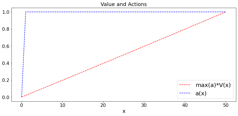
If \(p \geq 0.5\), then \(a(x) = 1\) for all \(x\) is optimal. One says that timid play is optimal when the game is favorable.
Proof:
Let \(U(x)\) be the probability of hitting \(F\) before \(0\) starting from \(x\) when choosing \(a(x) = 1\) for all \(x\). Then, the first step equations are
For \(p \neq q\), the solution can be verified to be
Also, when \(p > 0.5\), we claim that
To see this, note that the expression for \(U(x)\) shows that this inequality is equivalent to
Now, \(h(x) := (1/x - 1)^a\) is convex in \(x\), which implies that \(ph(p) + qh(q) \geq h((p+q)/2) = 1\).
This shows that \(U\) satisfies the DPE and also that \(a(x) = 1\) is optimal.
Unfortunately, the optimal strategy when \(p < 0.5\) is more complicated. We compute it below.
Notes:
Updates take time.
For clarity, we plot \(V(x) \times \max_y \{a(y)\}\) instead of \(V(x)\).
def dummy(Nd,pd):
    global N, p
    N, p = int(Nd), float(pd)

pd = widgets.Dropdown(options=['0.1', '0.2', '0.3', '0.4','0.5','0.6','0.7','0.8','0.9','1'],value='0.5',description='$p$',disabled=False)
Nd = widgets.Dropdown(options=['10', '30', '50', '70','100'],value='50',description='N',disabled=False)

z = widgets.interactive(dummy, Nd = Nd, pd = pd)
display(z)
def MDP1(p,F):  # How to gamble if you must
    t = np.arange(0,F+1)
    a = np.arange(0.0,F+1)
    V = np.arange(0.0,F+1)
    W = np.arange(0.0,F+1)
    q = 1 - p


    for x in range(F+1):  # initialize V
        V[x] = (x == F)
    S = 3*F
    W[F] = 1
    a[F] = 1
    for s in range(S):
        for x in range(1,F): # W = max_{1 <= u <= x} [p*V[x+u] + q*V[x-u]]
            y = 0.0
            for u in range(1,x+1):
                z = p*V[min(F,x+u)] + q*V[x-u]
                if z > y + 0.01:
                    a[x] = u
                    y = z
            W[x] = y
        V = W

    plt.figure(figsize = (14,6))
    pltV, = plt.plot(t,max(a)*V,'r--',label='max(a)*V(x)')
    plt.legend()
    pltV, = plt.plot(t,a,'b--',label='a(x)')
    plt.legend()
    plt.title('Value and Actions')
    plt.xlabel('x')

MDP1(p,N)